Music Source Separation – Pt.1 Background and Signal Basics
This series is inspired by my recent efforts to learn about a classic MIR task from end to end in a comprehensive way. This post is part 1, which focuses on the overall context and background of music source separation, along with some signal processing fundamentals. The series is inspired by the Music Source Separation tutorial at ISMIR 2020.
Background
-
Definition of music source separation: isolating individual sounds in an auditory mixture of multiple sounds
-
It is an undetermined problem - more required outcomes (guitar, piano, vocal) than observations (the mixture, 2 channels for stereo and 1 for mono).
-
Challenges compared to other source separation:
-
Music sources are highly correlated - all of the sources change at the same time.
-
Music mixing and processing are aphysical and non-linear due to signal processing techniques -> reverb, filtering, etc.
-
Quality bar is high for commercial use.
-
-
In music, it is assumed that sources and source types are known a priori.
Why Source Separation?
-
Enhance performance of the below tasks to do research on isolated sources than mixtures of those sources:
-
Automatic music transcription
-
Lyric and music alignment
-
Musical instrument detection
-
Lyric recognition
-
Automatic singer identification
-
vocal activity detection
-
fundamental frequency estimation
-
Relevant Fields
-
Speech separation (separate two speakers)
-
Speech enhancement (separate speech and noise)
- Any advancements in the two above can be used in music source separation with slight modifications
-
Beamforming - using spatial orientation of an array of microphones to separate sources. Researched separately from source separation, which has at most 2 channels.
Audio Representations
-
We are dealing with real signals and real data, we have Nyquist frequency and can only detect for up to half of its sampling rate.
-
Industry standards are either 44.1khz or 48khz.
-
To reduce computational load, deep learning source separation usually downsamples waveforms to 8-16kHz
-
-
Important Assumption!! Needs to keep sampling rate the same for training, validation, and test data
Note: Choose an Audio Representation that is easily separable
High-level steps
-
Convert the audio to a representation easy to separate
-
Separate the audio by manipulating the representation
-
Convert the audio back from the manipulated representation to get isolated sources.
- Invertability is important, artifacts will sound very obvious
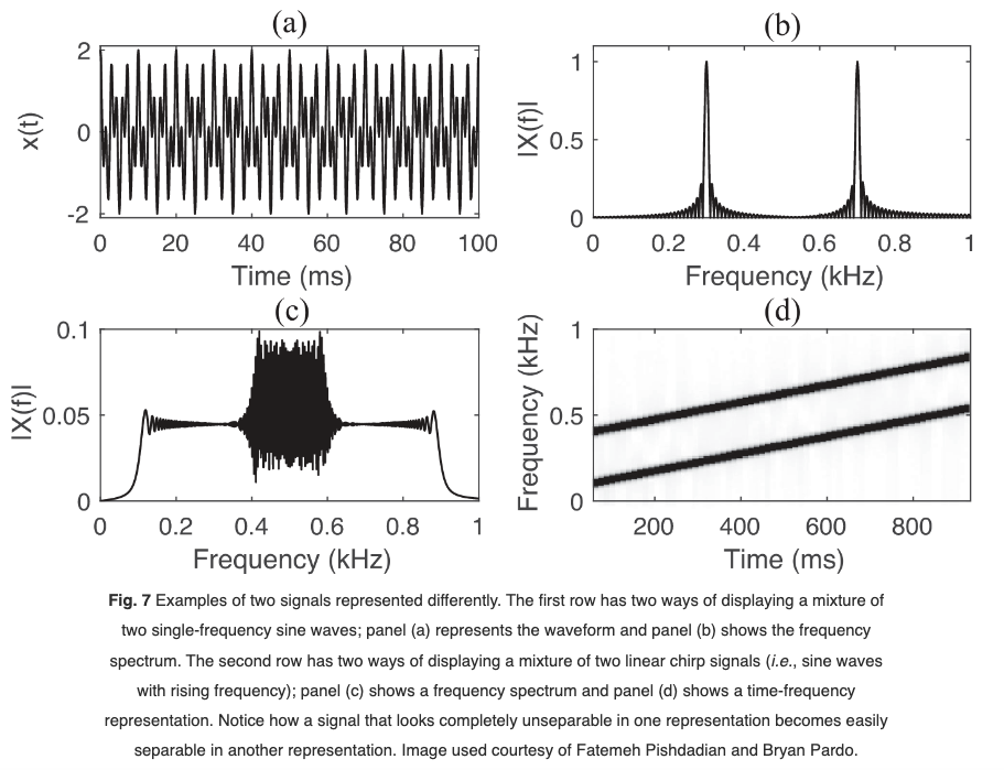
Time-frequency Audio Representations
STFT
-
Window types: blackman, triangle, rectangular, sqrt_hann, hann, etc.
-
Windows improve spectral resolution. We use it to reduce sidelobe levels in FT of a signal (an artifact, aka leakage)
-
In source separation tasks, usually sqrt_hann work the best.
-
-
Hop length vs Window length
-
Hop length: # of samples that the sliding window is advanced by at each step of the analysis (has effect on the time axis)
-
Window length: length of the short-time window (has effect on frequency axis, because the length of the short time window is equal to the number of frequency DFT can convert to, remember n=k in DFT)
-
-
Overlap-Add
- COLA (Constant Overlap-Add) is a setting where parameter sets that include window type, window length, hop length add up to a constant value, and allows the SFST to reconstruct the signal
-
Magnitude, Power, and Log Spectrograms
-
Magnitude spectrogram:for a complex valued STFT, the magnitude spectrogram is calculated by taking the absolute value of each element in the STFT, \(|X|\)
-
Power Spectrogram: \(|X|^2\)
-
Log spectrogram: \(log |X|\)
-
Log Power Spectrogram: \(log|X|^2\)
-
-
Mel spectrogram: spectrogram on a Mel scale to mimic human hearing.
-
Different source separation tasks might require different spectrograms, some require log whereas others are fine with magnitude and power
Output Representations
-
Some directly output waveforms, some output masks that were applied to the original mixture spectrogram and result is converted back to a waveform
-
If a waveform estimate for source \(i\) has already been obtained, then the mimxture sounds without source \(i\) can be obtained by subtracting the source waveform from the mixture waveform element-wise
-
Waveform vs TF Representation
-
Hard to say
-
SOTA usually use both as input, but speech separation has mostly converged upon using the waveform as input
-
Masking
-
Background
-
The number of masks = the number of sources you are trying to separate
-
Mostly masking works with TF representations, but some work also do masking on waveform-based
-
Masks are only applied to the magnitude values of a TF Representation and not the phase component
-
-
Definition
-
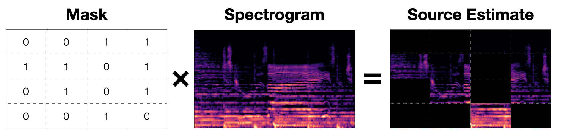
A matrix that is the same size as the spectrogram and contains values in [0.0, 1.0].
-
Mask application: element-wise multiplication (Hadamard product \(\odot\)) of the mask to the spectrogram.
-
For each source \(i\), we can estimate the source with the estimated mask \(\hat{M_i}\) and the magnitude spectrum \(|Y|\), where \(|Y|\) is the STFT, and \(Y \in \mathbb{C} ^{T\times F}\)
\[S_i = \hat{M_i} \odot |Y|\] -
This means, if we add up the masks for all the sources element-wise, we should obtain a matrix of all ones, \(J \in [1.0]^{T \times F}\)
- In other words, \(J = \sum_{i=1}^N \hat{M_i}\)
-
-
Binary Masks
-
Binary masks are masks where the only values the entries are allowed to take is 0 or 1. This makes the assumption that any TF bin in the M matrix will only have one source present, because J is a matrix of all ones. If we have more than one source present, J will be greater than 1, which does not make sense.
- In literature, this is called W-disjoint orthogonality
-
We don’t use this to produce final source estimates, but they are useful as training targets, especially with NN models like Deep Clustering
-
-
Soft Masks
-
Masks are allowed to take any value within the interval [0.0, 1.0]. We assign part of the mix’s energy to a source, and the other parts to other sources.
-
This makes soft masks more flexible and closer to the reality - it is not very often that all of the energy in a mixture are assigned to only one source.
-
-
Ideal Masks
-
An Ideal Mask or an Oracle Mask, represents the best possible performance for a mask-based source separation approach.
-
Needs access to the ground truth
-
Usually used as an upper limit on how well a source separation can do
-
Some waveform-based approaches for speech separation have surpassed the performance of Ideal Masks
-
Phase
-
Phase is also important to model, on top of creating better mask estimates that are related to magnitude components of a wave.
-
Sinusoid:
-
Formulaic Definition: \(y(t) = Asin(2\pi ft + \phi)\)
-
When \(\phi \neq 0\), the sinusoid will be shifted in time to the left (“advancing”) by \(-\frac{\phi}{2\pi f}\)
-
Proof:
Let \(t_\delta = t_\phi - t\)
Before \( \phi, y(t) = Asin(2\pi ft)\)
After \(\phi, y(t_{\phi}) = Asin(2\pi ft_{\phi} + \phi)\)
We want to know how much time has shifted, so we really just care about \(t_\delta\). To shift is to mean that the y value at time t for y(t) is the same as the y value at \(t_\phi\) for \(y(t_\phi)\)
\(Asin(2\pi ft) = Asin(2\pi ft_\phi + \phi)\)
\(2\pi ft = 2\pi f(t +t_\delta) + \phi\)
\(t_\delta = - \frac{\phi}{2\pi f}\)
-
-
Why don’t we model phase usually?
-
Phase is sensitive to noise compared to magnitude and the wave is sensitive to the changes in frequency and initial phase
-
Humans don’t always perceive phase differences
-
-
How to Deal with Phase:
-
The Easy Way - Noisy Phase
-
Copy the phase from mixture - the mixture phase is also referred to as the noisy phase.
-
Not perfect but works surprisingly well
-
Wave-U-Net has a whole paragraph on this
-
Reconstructing the signal with Noisy Phase:
-
Magnitude spectrum: \(\hat{X_i} = \hat{M_i} \odot |Y|\)
-
To reconstruct the signal, use IFT (Inverse Fourier Transform):
\[\tilde{X_i} = (\hat{M_i} \odot |Y|) \odot e^{j \dot \angle{Y}}\]
-
-
-
The Hard Way Pt.1 - Phase Estimation
-
Griffin-Lim algorithm
-
Reconstructs the phase component of a spectrogram by iteratively computing an STFT and an inverse STFT. Usually converges in 50-100 iterations
-
Can still leave artifacts in the audio
-
Librosa has an implementation
-
-
MISI (Multiple Input Spectrogram Inversion)
-
a variant of Griffin-Lim made specifically for multi-source source separation
-
Adds an additional constraint to the original algo s.t. all of the estimated sources with estimated phase info add up to the input mixture
-
-
The STFT & iSTFT computations + the phase estimation algorithms are all diffrentiable and can be used in neural networks and train directly on waveforms, even when using mask-based algorithms.
-
-
The Hard Way Pt.2 - Waveform Estimation
-
Recently, a lot of deep learning based models are end to end with input and output both as waveforms - the model decides how it represents phase.
-
Might not be most efficient or effective, but there are research being done
-
-