Transformers Explained with NLP Example
Transformers is a sequence-to-sequence model that relies heavily on attention mechanism without recurrence or convolutions. It is proposed by Google Researchers’ in their paper Attention is All You Need.
In this post, we will look at the model architecture and break down the main concepts of Transformers below:
- Positional Encoding
- Attention mechanism used in transformers (sub-bullets not mutually exclusive):
- Scaled Dot-Product Attention
- Self Attention
- Encoder-Decoder Attention
- Multi-Head Attention
- Masked Attention
- Scaled Dot-Product Attention
- Residual connections
- Layer Normalization
High-Level Model Architecture
We will go through the high-level model architecture and treat each concept as a black box first. The later sections will go over each concept one by one.
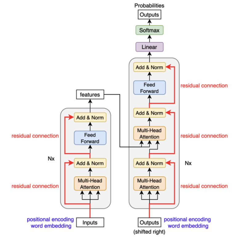
The transformers are composed of N=6 encoder blocks and N=6 decoder blocks. We’ll call the left half of the architecture below input & encoding, the right half output & decoding.
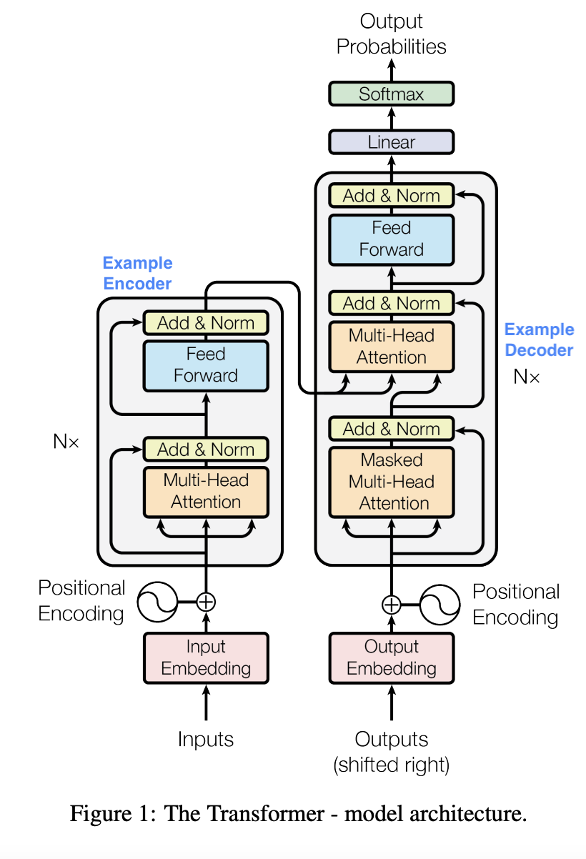
Input & Encoding (left side)
The text input gets tokenized and the tokens get converted into vectors of a certain length (in the paper, \(d_{model}\) = 512) through learned embedding (i.e. the transformer learn this embedding from scratch). These input vectors will have positional encoding added to them to keep track of their position in the input sentence before they enter the encoder blocks.
There are two main parts in an encoder block: self-attention and feedforward neural network.
- Self attention looks at the dependencies against all other words in the input sentence as it encodes the current word. For example, for the sentence “The animal didn’t cross the street because it was tired”, the model will associate “The” and “Animal” with “it” when it is encoding the word “it”.
- The feed-forward neural network will take the self-attention output and add element-wise non-linearity transformation to the encoder. For more explanation, please refer to this stackexchange thread I found useful. My recommendation is to read it once you understood what self attention and multi-head attention means.
The residuals connections and layer normalization (the Add & Norm box in the model architecture diagram) is not specific to the encoders and on a high level it is added there for better model performance to achieve the same accuracy faster and to avoid the exploding or vanishing gradient problem. We will go through those later in details.
As mentioned previously, there are 6 encoder blocks of the same structure that have different weights. The input vectors go through all 6 encoder blocks before they are connected with the decoding side.
Encoder-Decoder Attention
The output vectors from the 6 encoder blocks will be connected with each decoder block through encoder-decoder attention (cross-attention). Attention mechanisms have query, key, and vectors (to be explained later). The keys and values come from the output of the encoder blocks, while the queries come from the target sequence. The encoder-decoder attention gives the ongoing output context of the input sentence.
Output & Decoding (right side)
The output & decoding side outputs one word at each time step and each output word will be sent back for processing in order to output the word for the next time step.
For each time step, the translated output will go through 6 decoder blocks first.
Each decoder block is composed of three parts:self attention, encoder-decoder attention, feed-forward neural network.
- Self attention here uses masking, meaning that it will temporarily hide the words after the current time step.
- For example, if we are translating “The animal didn’t cross the street because it was tired (动物没有穿过街道因为它很累)” and we only processed up to “动物没有”, then we will only check the dependencies between the first four translated characters.
- Encoder-decoder attention is mentioned in the section right above. It is worth noting that the encoder ouputs are leveraged in each of the decoder block.
- Feed-forward network to add nonlinearity
After the 6 decoder blocks, the output goes through a linear and softmax layer to output the final word. The linear layer is a fully connected layer that projects our decoder stack vectors to a very large logits vector, that has the same length as the number of our vocabulary size. Each cell of the logits vector corresponds to a word. The softmax function will be applied onto the logits vector to select the most likely word to be output. Then the final word is fed back to the right side to generate the next word, until we reach the end of the sentence.
Positional Encoding
Since the transformers don’t have recurrence or convolutions, they chose positional encoding as a mechanism to keep track of the position of each word in the sequence.
On a high level, positional encodings are fixed numbers added to each element of the word embedding vectors. They are vectors of the same size as word embeddings (\(d_{model}\) = 512).
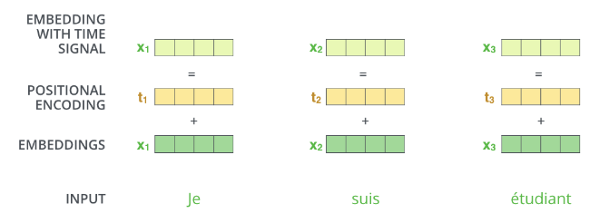 Source: The Illustrated Transformer
 These encodings depend on both the position of the word and the index of the vector, and are defined with sine for even index and cosine for odd index.
\[PE_{pos, 2i} = sin(pos/10000^{2i/d_{model}})\] \[PE_{pos, 2i+1} = cos(pos/10000^{2i/d_{model}})\]Let’s visualize the positional encodings for each word position and each encoding dimension.
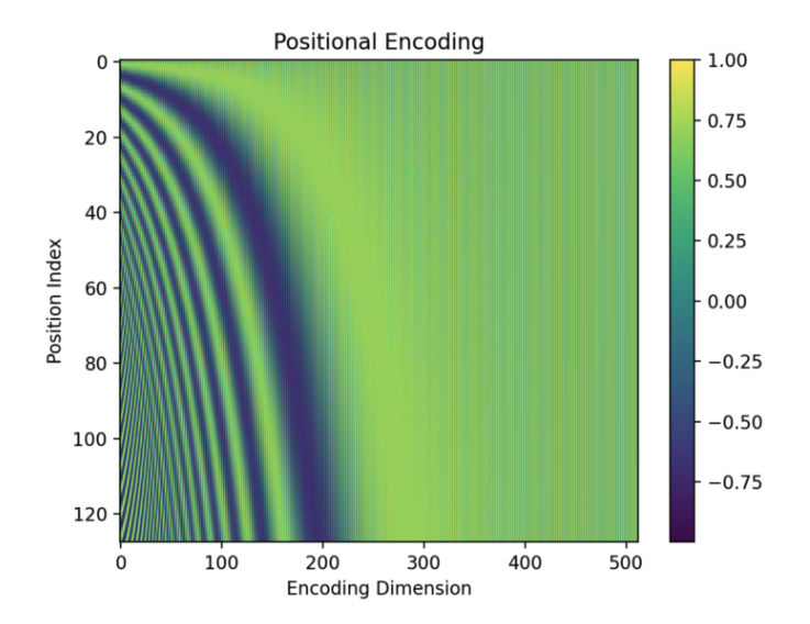 Visualization of positional encodings for 128 words. Each encoding vector has 512 dimensions. Source: kikaben
Let’s zoom in and take a closer look at the value for each dimension. We will see as index nears the end, the cosine values will go closer to 1 and the sine values will go closer to 0, which is why there is an alternating pattern on the right side of the graph that is hard to see on the zoomed out version.
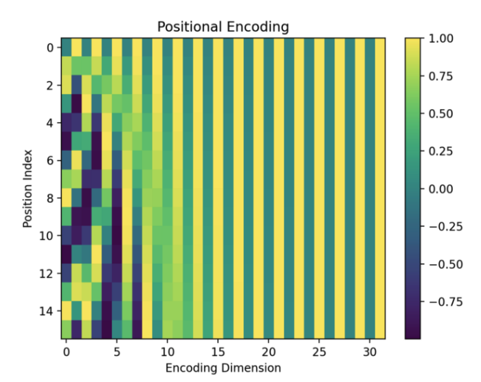 A Zoomed In Version. Source: kikaben
 Here is the encodings with the numbers plugged into the formula definition:
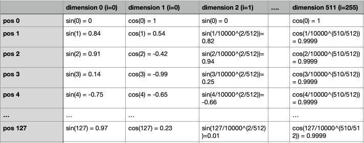 Example Encoding Values. Source: author
 In the zoomed out graph, we can clearly see that the positional encoding vector for each position is unique. Each dimension of the positional encoding corresponds to a sinusoid. For example, dimension 0 is a sinusoid of \(sin(pos)\).
The model is able to keep the encoding throughout the entire architecture because of the residual connections. (Feel free to skip to the residual connections section to understand what it is.) If you are curious to learn morer about the positional encoding, I refer you to this post by kikaben.
 Source: kikaben
 Attention Mechanism
Now that we have a high-level idea of what the model architecture looks like, let’s dive into the core concept behind transformers – attention. Attention is designed to mimic cognitive attention and learns which part of the data is more important than the other depending on context.
Scaled Dot-Product Attention
Dot product attention consists of queries and keys (both of dimension \(d_k\)) and values of dimension \(d_v\).
You can think of query as the word that we are trying to assess the similarity of against words in a sequence and keys are the words in that sequence. Values and keys share the same index/position, but is a different extraction of the word. Queries, keys, and values are all calculated/learned from the the initial embedding (x) by the model.
Self attention and encoder-decoder attention both use scaled dot-product attnetion, and are very similar in nature. In self attention, queries, keys, and values all come from the input sequence. However, in encoder-decoder attention, queries come from the target sequence and keys and values come from the input sequence.
Below we use self attention as an example. For simplicity, the input sequence we are looking at is “Thinking Machines”.
Self Attention
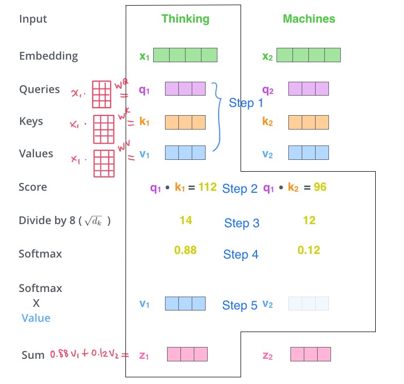 Scaled Dot-Product Self Attention. Source: The Illustrated Transformer, modified by author
 Step 1. Learn the query, key, value vectors from the input embedding
There is no strict rule on the exact dimension of query, key, value vectors. In the original paper, the authors went with \(d_k = 64\). The model extracts the vectors through three weight matrices \(W^Q, W^K, W^V.\)
Then we get ready to calculate the attention. For reference, the attention is defined as below. In the
\[Attention(Q,K,V) = softmax(\frac{QK^T}{\sqrt{d_k}})V\]Step 2. Score each word through dot product We take the dot product of the query (\(q_1\), current word) and all the words in the sequence (\(k_1\) and \(k_2\)) to get a score that tells us how much focus the model should place on any word in the sequence when it is processing the current word.
Step 3. Scale the dot product by \(\sqrt{d_k}\)
The paper itself explained the reason quite clearly,
We suspect that for large values of \(d_k\), the dot products grow large in magnitude, pushing the softmax function into regions where it has extremely small gradients. To counteract this effect, we scale the dot products by \(\frac{1}{\sqrt{d_k}}\).
To illustrate why the dot products get large, assume that the components of q and k are independent random variables with mean 0 and variance 1. Then their dot product, \(q·k = \sum^{d_k}_{i=1}q_ik_i\), has mean 0 and variance \(d_k\).
Step 4. Take softmax of the scaled dot products. This step converts the dot products into normalized scores that add up to 1.
Step 5. Multiply the softmaxed score with value. This step gives us a weighted value vector that tells the model how much information the current word should have from other words, and for the last step, we add up all the weighted value vectors.
Step 6. Sum each elements of the softmaxed value vector together to get the final output vector. The last step gives us the output of the attention mechanism. Note that even though we took the dot product of the current processing word with each word in the sequence, there is only one output vector for each word after element-wise summation of step 6.
Multi-Head Attention
Now that we know how scaled dot product attention works, the rest should be a breeze. They are modification to the original dot product attention to allow the model to perform better.
The first one is multi-head attention. Different words have different meanings in the same sentence, so only learning one representation of the word is not enough. Transformer proposes to learn h key, value, query vectors that are smaller in dimension for the same word (i.e. split the original attention mechanism into h attention heads) and perform the attention mechanism on each set of these k,v,q vectors. These attention functions can be run in parallel and in total, the attention mechanism will be run h times for each multi-head attention mechanism.
The specification in the paper is, there are 8 parallel attention layers (i.e. heads), and each key, value, query vectors have the dimension of 64 (\(d_{model}/h = 512/8\)). The dimension of the key, value, query vectors for each head does not need to follow exactly like the original paper, and it doesn’t need to be equal to \(d_{model}\) after multiplying with h. In order to return a vector that the model can continue training on with the following steps, we concatenate the output vectors from the 8 heads and apply an output weight matrix \(W^O\). To quote the original formula in the paper:
\[MultiHead(Q,K,V) = Concat(head_1, ..., head_h)W^O\] \[where\space head_i = Attention(QW_i^Q, KW_i^K, VW_i^V)\]where the projections are parameter matrics \(W_i^Q \in \mathbb{R}^{d_{model}\times d_k}\), \(W_i^K \in \mathbb{R}^{d_{model}\times d_k}\), \(W_i^V \in \mathbb{R}^{d_{model}\times d_v}\) and \(W_i^O \in \mathbb{R}^{dhd_v\times d_{model}}\).
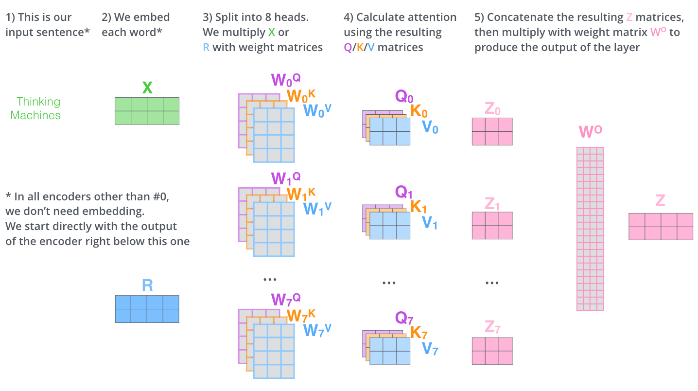 Multi-head attention. Source: The Illustrated Transformer
 Masked Attention
Masked attention means that the attention mechanism receives inputs with masks on and does not see the information after the current processing word. This is done by setting attention scores to negative infinity to the words behind the current processing word. Doing so will result in the softmax assigning almost-zero probability to the masked positions. Masked attention only exists in decoder.
As we move along the time steps, the masks will also be unveiled:
(1, 0, 0, 0, 0, …, 0) => (<\SOS>)
(1, 1, 0, 0, 0, …, 0) => (<\SOS>, ‘动’)
(1, 1, 1, 0, 0, …, 0) => (<\SOS>, ‘动’, ‘物’)
(1, 1, 1, 1, 0, …, 0) => (<\SOS>, ‘动’, ‘物’, ‘没’)
(1, 1, 1, 1, 1, …, 0) => (<\SOS>, ‘动’, ‘物’, ‘没’, ‘有’)
Add & Norm Layers
Residual Connection (the Add)
Residual connections were first introduced in ResNet, a convolutional neural network that won a number of major image classification challenges at that time. It was introduced to combat vanishing gradients caused by the depth of the network. The deeper the network, the more vulnerable it is to vanishing or exploding gradients. The residual connection avoids this problem – in a conventional neural network, the output of the previous layer gets fed into the next layer as input, whereas the residual connections provide the output of the previous layer another path to reach latter parts of the network by skipping some layers, as shown in the diagram.
Here F(x) refers to the outcome of layer i through layer i + n. In the example here, residual connection first applies the identity matrix to the input at layer i and then performs element-wise addition of F(x) and the outcome of the identity matrix operation x. The operation on the input at layer i (x) does not have to be identity matrix, it could also be more complicated operations. For example, if the dimensions of F(x) and x do not match, the operation could be a linear transformation on x.
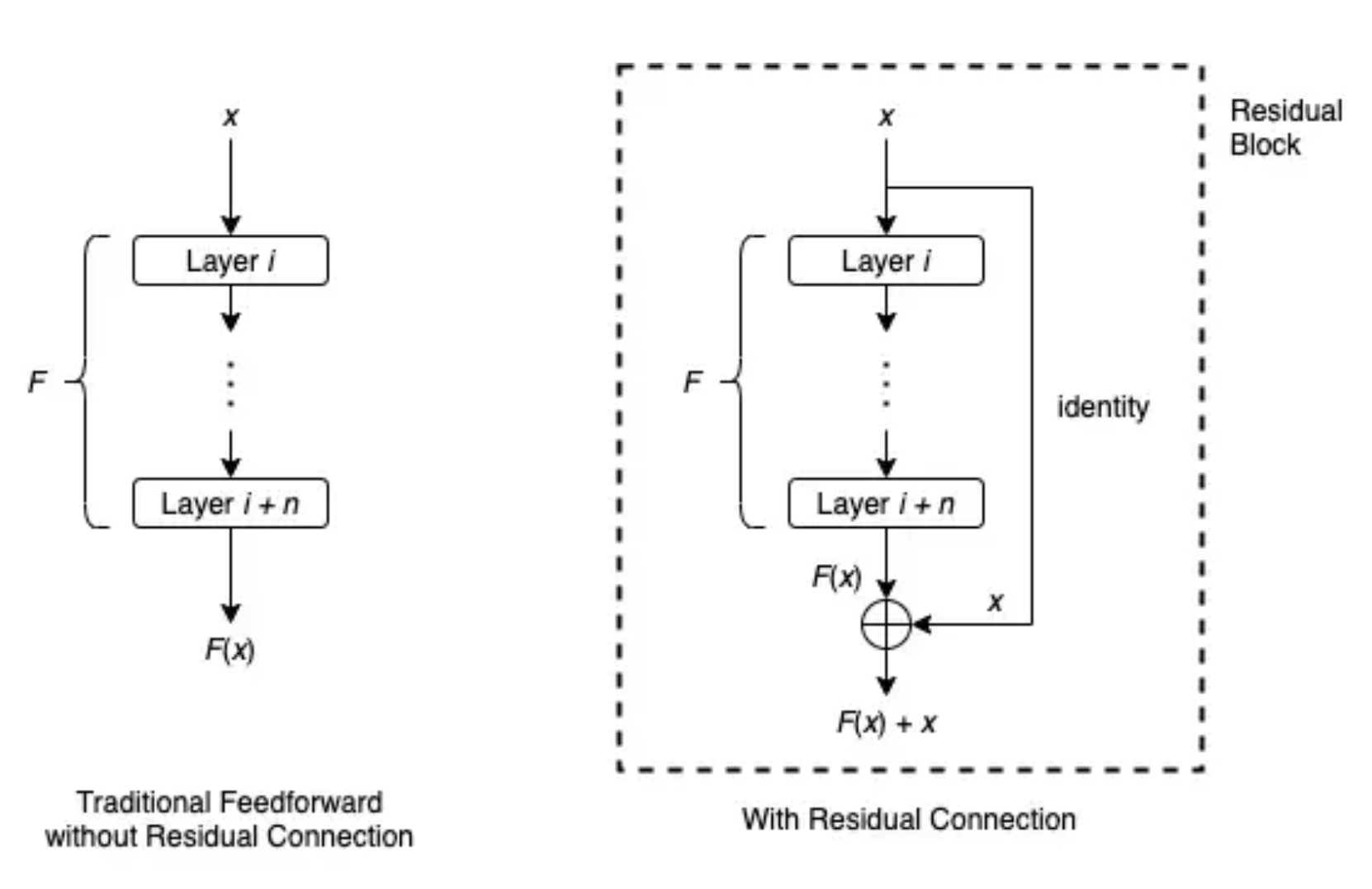 Residual Block. Source: Wanshun Wong
 Residual connections can be added to each layer. In the Transformer model, a residual connection is employed around each of the two sub-layer (i.e. attention layer and feedforward neural network layer) in each encoder and decoder block.
Layer Normalization (the Norm)
To understand what a layer normalization is, let’s take a look at its sibling, batch normalization.
Batch Normalization
Goal & Benefit
- It is used to convert different inputs into similar value ranges.
- Each epoch takes longer to train due to the amount of computations but overall the convergence of the model will be faster, and takes less epochs.
- Batch normalization allows the model to achieve the same accuracy faster, so performance can be enhanced with the same amount of resources.
- No need to have a separate standardization layer, where all the input data is transformed to have mean 0 and variance 1.
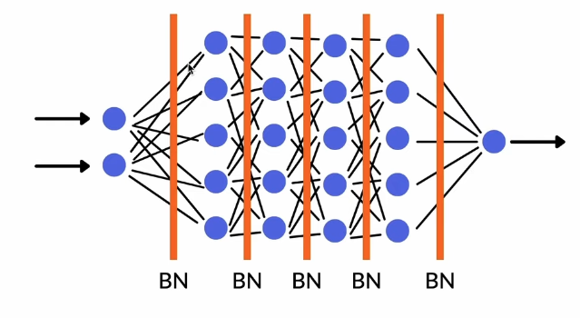 Batch Normalization Placement
 Process
- Standardize the input data so that they all have mean 0 and variance 1
- Train the layer to transform the data into another range
- In the graph below, \(\hat{x}^{(i)}\) is the standardized values from step 1
- \(\beta\) is offset
- \(\gamma\) is scale
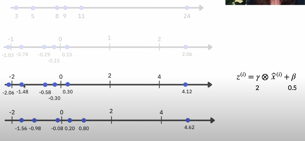 Batch Normalization Transformation
 Layer Normalization
Batch normalization is hard to use because they are very dependent on batches. So layer normalization is introduced - it is the same process but instead of standardizing the data across batches as shown in figure A, it standardizes the data across layer as shown in figure B.
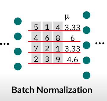
Figure A. Batch Normalization
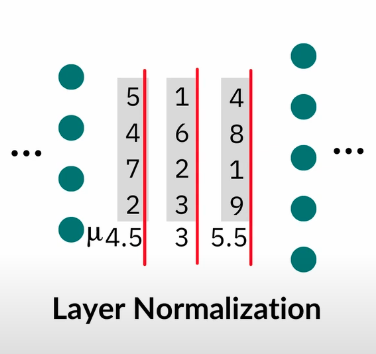
Figure B. Layer Normalization
So if we were to visualize the Add & Norm layer, it woud look something like this:

Congrats! You’ve learned the basic concepts of the Transformer, now you can try out the code implementation in Tensorflow :)
Resources
- The Illustrated Transformer by Jay Alammar
- The Annotated Transformer by Harvard NLP
- Glass Box ML Transformer explained by Rachel Draelos