Intro to Generative Adversarial Network with Speech Enhancement Paper Example
Generative Adversarial Network, 2014
Machine Learning Course by Google Developers here
-
Definition (high level): create new data instances that resemble your training data
-
High level working mechanism: GANs achieve this level of realism by pairing a generator, which learns to produce the target output, with a discriminator, which learns to distinguish true data from the output of the generator. The generator tries to fool the discriminator, and the discriminator tries to keep from being fooled.
- See the diagram below
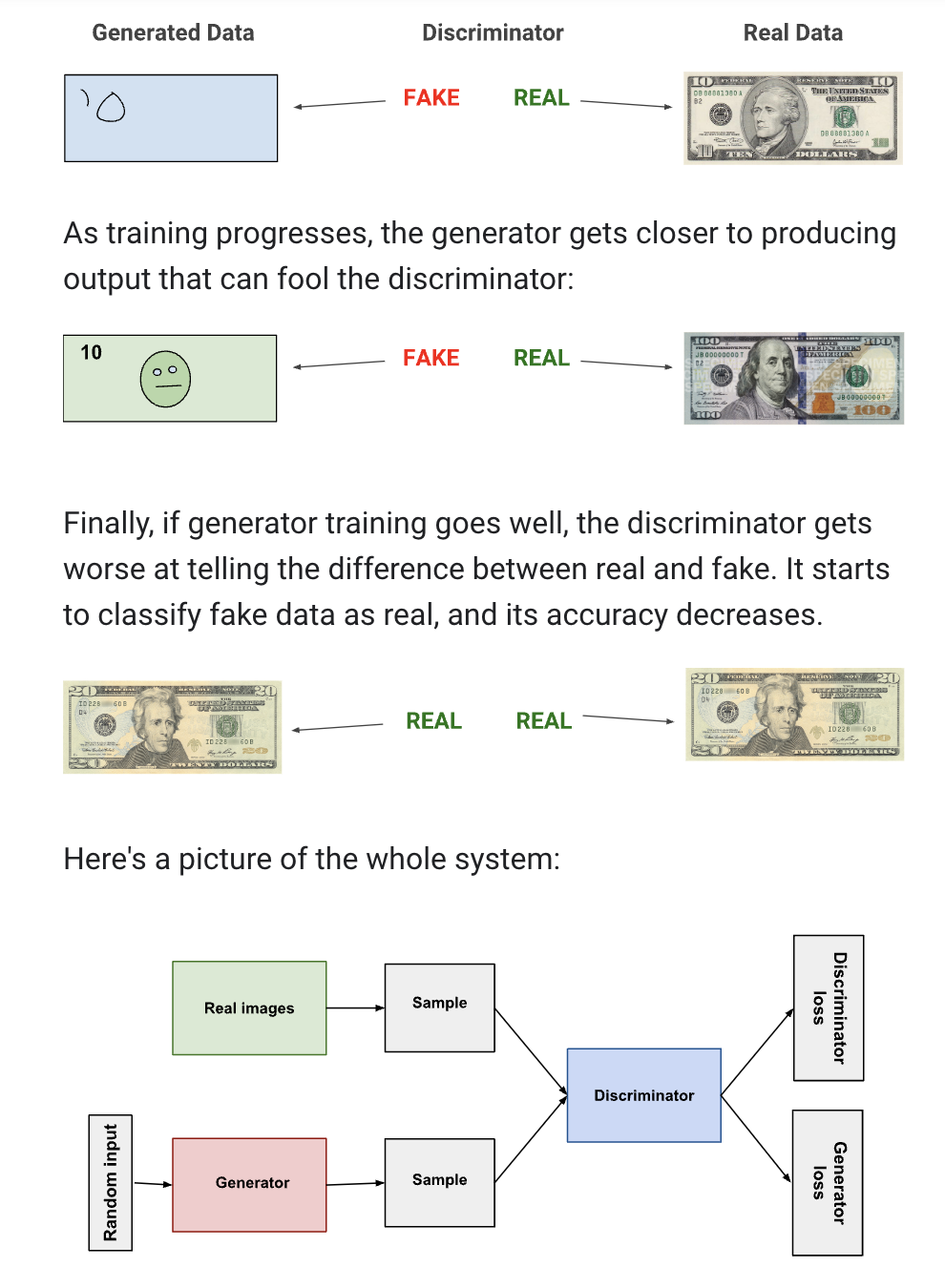
- See the diagram below
Step 1. Discriminator trains for one or more epochs.
The discriminator takes input from real images and the fake images the generator outputs, update its weights through backpropagation to distinguish between real and fake data.
Generator does not update its weight during this period, and discriminator ignores generator loss in this round. 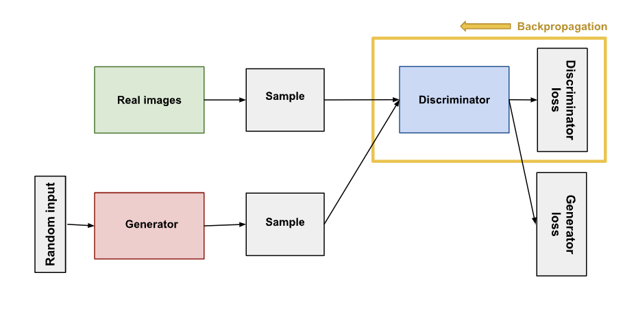
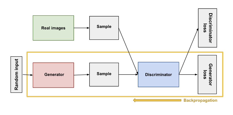
Step 2. Generator trains for one or more epochs.
-
Goal is to generate data that the discriminator will classify as real, so the generator loss penalizes the generator for failing to fool the discriminator.
- This requires the generator training to incorporate discriminator. How it involves discriminator is using it to feed it the generator output and derive the generator loss.
-
When generator trains, discriminator stays put and does not update weights.
-
Procedure:
-
Sample random noise that we feed into the generator. The generator will transform this into meaningful output
- the distribution of the noise doesn’t matter much; could also be non-random input
-
Produce generator output from sampled random noise
-
Get discriminator’s Real or Fake classification for generator output
-
Calculate loss from discriminator classification (generator loss)
-
Backpropagate through both the discriminator and generator to obtain gradients
-
Use gradients to change only the generator weights.
-
Step 3. Repeat step 1 and 2 to alternate training
-
Convergence: when discriminator classification has a 50% accuracy (it can’t tell between a true and a fake)
-
This poses a problem: if discriminator feedback becomes 50% (near random), then the generator is training on useless feedback, which in turn affects its own quality
-
GAN convergence is a fleeting, instead of stable, state
-
Loss Functions
-
Goal: capture the difference between the distributions of “real” data and “fake” data generated by the generator
-
Still ongoing research
-
Example: minimax loss (used in og GAN paper), Wasserstein loss (used for TF-GAN estimator)
-
-
Minimax Loss:
-
It’s the same formula that the discriminator and generator are optimizing over. Discriminator maximize, generator minimize
Ex[log(D(x))]+Ez[log(1−D(G(z)))]
In this function:
-
D(x)is the discriminator’s estimate of the probability that real data instance x is real. -
Ex is the expected value over all real data instances.
-
G(z)is the generator’s output when given noise z. -
D(G(z))is the discriminator’s estimate of the probability that a fake instance is real. -
Ez is the expected value over all random inputs to the generator (in effect, the expected value over all generated fake instances G(z)).
-
The formula derives from the cross-entropy between the real and generated distributions.
The generator can’t directly affect the
log(D(x))term in the function, so, for the generator, minimizing the loss is equivalent to minimizinglog(1 - D(G(z))). -
-
Caveat-> Vanishing Gradients
-
The generator can fail due to vanishing gradients and the GAN might get stuck in the early stages if the discriminator is too good. Two remedies:
-
Modified minimax loss: the original paper suggests to modify the generator loss so that the generator tries to maximize log D(G(z))
-
Wasserstein loss introduced below is designed to prevent vanishing gradients
-
-
-
-
Wasserstein Loss
-
! Modification of GAN Scheme: discriminator does not classify instances or produce probabilities, but instead it produces a number. We call it critic instead of discriminator
-
For real instances: outputs a really big number
-
For fake instances: outputs a really small number
-
Requires the weights throughout GAN to be clipped so that they remain within a constrained range
-
-
Critic Loss: D(x) - D(G(z))
- The discriminator maximizes this function, they want the difference between the real and the fake to be as big as possible
-
Generator Loss: D(G(z))
- The generator maximizes this function because they want the discriminator to think what they generated is a real instance
-
D(x)is the critic’s output for a real instance. -
G(z)is the generator’s output when given noise z. -
D(G(z))is the critic’s output for a fake instance. -
The output of critic D does not have to be between 1 and 0.
-
The formulas derive from the earth mover distance between the real and generated distributions.
-
WassersteinGANs is less vulnerable to getting stuck than minimaxGANs, and avoid problems with vanishing gradients
-
Common Problems
-
Vanishing Gradients:
- If discriminator is too good, the generator training can fail due to vanishing gradients. Remedy is through 1) Wasserstein loss 2) modified minimax loss
-
Mode collapse: usually happens when the discriminator gets stuck in local minima.
-
Mode collapse describes the scenario where each iteration of generator over-optimizes for a particular discriminator, so the generators rotate through a small set of output types. This is against what we want: for generator to produce a wide variety of outputs.
-
Remedy:
-
Wasserstein loss: designed to avoid vanishing gradient/discriminator being stuck in a local minima
-
Unrolled GANs: uses a generator loss function that not only incorporates the current discriminator’s classification, but also the outputs of future discriminator versions.
-
-
-
Failure to convergence: discriminator can’t tell the diff between real and fake, so generator trains on junk feedback. Two remedies:
-
Adding noise to discriminator inputs
-
Penalizing discriminator weights
-
GAN Application in Speech Enhancement
Here the examples are based on the series of high fidelity speech denoising and dereverberation work done by Prof. Adam Finkelstein’s lab.
- HiFi-GAN: High-Fidelity Denoising and Dereverberation Based on Speech Deep Features in Adversarial Networks. Project page link
- Based on deep features
- HiFi-GAN2: Studio-quality Speech Enhancement via Generative Adversarial Networks Conditioned on Acoustic Features. Project page link
- Based on deep features but also includes a prediction network for acoustic features before training the GAN
High-level Takeaway:
HiFi GAN
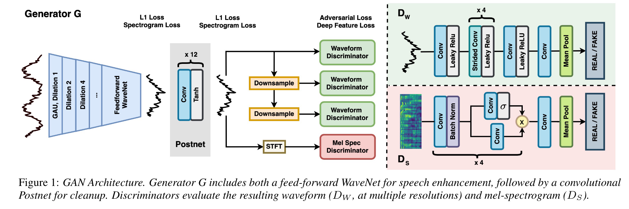
HiFi GAN builds on top of the lab’s previous work of joint denoising and dereverberation on a single recording environment, and is able to generalize to new speakers, speech content, and environments. The model architecture at a glance:
- Generator:
- Uses a WaveNet architecture (dilutated CNN), which enables a large receptive field for additive noise and long tail reverberation.
- Uses log spectrogram loss, L1 sample loss.
- Combined with postnet for cleanup
- 4 Discriminators:
- Wave discriminator (time domain):
- 3 waveform discriminators operating at 16kHz, 8kHz, and 4kHz resepctively.
- They use the same network architecture but do not share weights
- Spectrogram discriminator (time frequency domain):
- Sharpens the spectrogram of predicted speech
- Having two discriminators stablize the training and make sure that no single type of noise or artifact gets overaddressed
- The generator is penalized by adversarial losses, and deep feature matching losses computed on the feature maps of the discriminators.
- Deep feature loss prevents the model from mode collapse (where the model only produces monotonous examples)
- Wave discriminator (time domain):
HiFi-GAN2
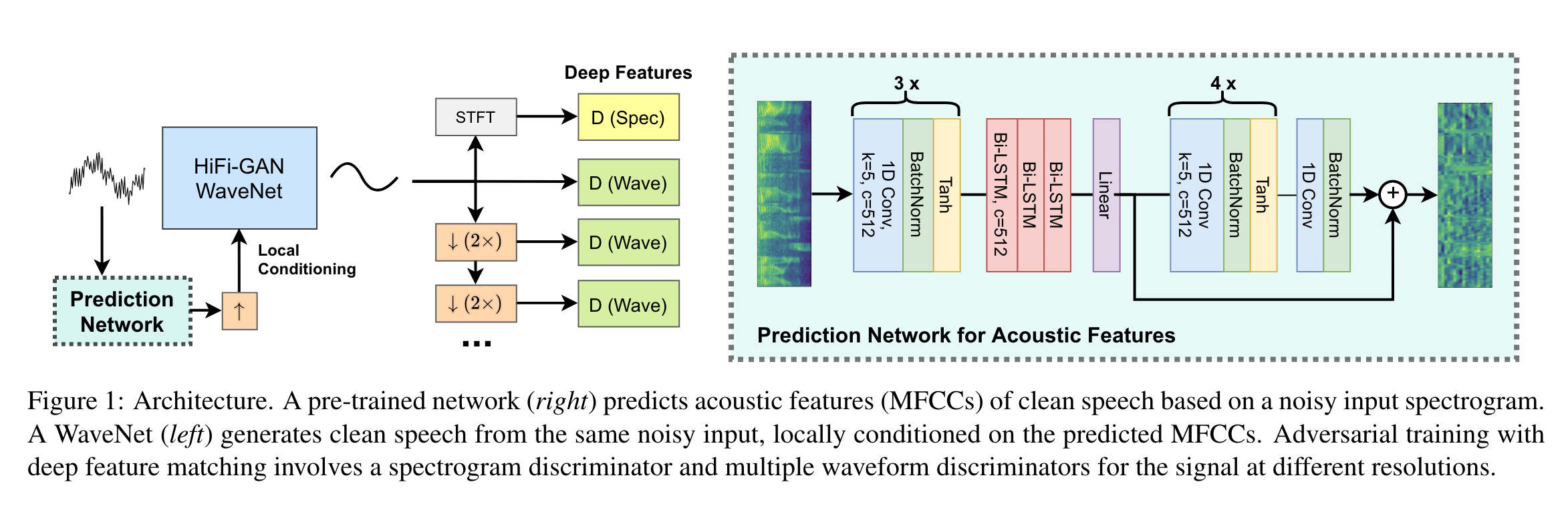
HiFiGAN2 is conditioned on acoustic features of the speech to achieve studio quality dereverberation and denoising.
- Improvement Areas of HiFi-GAN:
- Inconsistency in speaker identity when noise and reverb are strong.
- Ambiguity in disentangling speech content and speaker identity from environment effects
- WaveNet still has a limited receptive field and lack of global context.
- Inconsistency in speaker identity when noise and reverb are strong.
- HiFi GAN2 Proposal:
- Condition the WaveNet on acoustic features that contain clean speaker identity and speech content information
- Incorporate a recurrent neural network to predict clean acoustic features from the input noisy reverberant audio, which is then used as time-aligned local conditioning for HiFi GAN.
- RNN trained using MFCC (more robust to noise than Mel spectrogram) of simulated noisy reverberant audio as input and MFCC of clean audio as target
HiFi GAN Paper Notes
Introduction
Existing research done
-
Traditional signal processing methods (Wiener filtering, etc.):
-
time-frequency domain
-
generalize well but result not good
-
-
Modern machine learning approaches:
-
transform the spectrogram of a distorted input signal to match that of a target clean signal
-
1) estimate a direct non-linear mapping from input to target
-
2) mask over the input
-
-
Use ISTFT to obtain waveform, but can hear audible artifacts
-
Recent advances in time domain
-
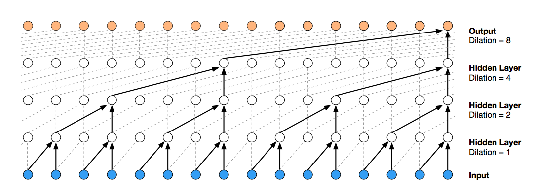
WaveNet (time domain): leverages dilated convolution to generate audio samples. Due to dilated convolution, it is able to zoom out to a broader receptive field while retaianing a small number of parameters.
-
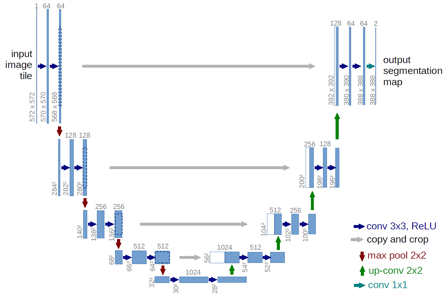
Wave-U-Net: leverages U-Net structure to the time domain to combine features at different
-
U-Net is a CNN that has encoder-decoder structure that separates an image into different sources / masks
-
Have their own distortions, sensitive to training data and difficult to generalize to unfamiliar noises and reverberation
-
-
From the perspective of metrics that correlate with human auditory perception:
-
Optimizing over differentiable approximations of objective metrics (closely related to human auditory perception) like PESQ and STOI: reduce artifacts but not significantly -> Metrics correlate poorly with human perception at short distances
-
Deep feature loss that utilize feature maps learned for recognition tasks (ex. denoising):
-
underperform with different sound statistics (paper proposal is to address this with adversarial training)
-
What is deep feature loss? (using image an example) The deep feature loss between two images is computed by applying a pretrained general-purpose image classification network to both. Each image induces a pattern of internal activations in the network to be compared, and the loss is defined in terms of their dissimilarity.
-
-
Paper Proposal:
-
WaveNet architecture
-
Deep feature matching in adversarial training
-
On both time and time-frequency domain
-
Discriminators used on waveform sampled at different rates and on mel-spectrogram. They jointly evaluate the generated audio -> this way the model generalizes well to new speakers and speech content
Method
-
Builds on previous work: perceptually-motivated environment-specific speech enhancement.
-
Previous work aims at joint denoising and dereverberation on single recording environment
-
Goal now is to generalize across environment
-
-
Uses WaveNet for speech enhancement (work by Xavier)
- Non-causal dilated convolutions with exponentially increasing dilation rates, suitable for additive noise and long tail reverberation.
-
Uses log spectrogram loss and L1 sample loss
- there are 2 spectrogram losses at 16kHz: 1 with large FFT window and hop size (more frequency resolution), 1 with small FFT window and hop size (more temporal resolution)
Postnet
-
attach 12 1D convolutional layers, using Tanh as an activation function.
- Attaches the L1 and spectrogram loss to both output of main network before postnet and after postnet. Postnet cleans up the coarse version of the clean speech generated by main network
Adversarial Training
-
The generator is penalized with the adversarial losses as well as deep feature matching losses computed on feature maps of the discriminators
-
Multi-scale multi-domain discriminators
-
Waveform discriminator operating at 16khz, 8khz, and 4khz for discrimination at different frequency ranges.
- They share the same network architecture but not the weights
-
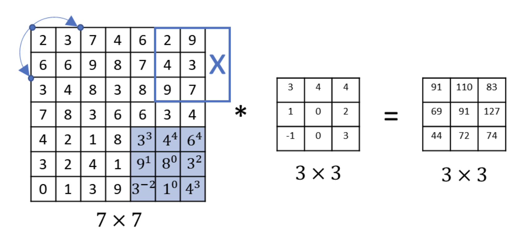
Composed of strided convolution blocks (see actual diagram)
- Strided convolution: the stride is 2 in the picture below. It means you skip a certain length when you are sliding the filter.
- Strided convolution: the stride is 2 in the picture below. It means you skip a certain length when you are sliding the filter.
-
Other Relevant Work wrt HiFiGAN:
- Perceptually-motivated Environment-specific Speech Enhancement: link
- Joint denoising and dereverberation on single recording environment
- Bandwidth Extension is All You Need: link
- Extending 8-16kHz sampling rate to 48kHz
- MUSIC ENHANCEMENT VIA IMAGE TRANSLATION AND VOCODING link
- High fidelity instrument enhancement also with a GAN