Deep Learning for Music Information Retrieval – Pt. 4 (RNN, Seq2Seq, Attention)
This series is inspired by my recent efforts to learn about applying deep learning in the music information retrieval field. I attended a two-week workshop on the same topic at Stanford’s Center for Computer Research in Music and Acoustics, which I highly recommend to anyone who is interested in AI + Music. This series is guided by Choi et al.’s 2018 paper, A Tutorial on Deep Learning for Music Information Retrieval. I’d like to give a shoutout to Chris Olah’s wonderful explanation on LSTM as well.
It will consist of four parts: Background of Deep Learning, Audio Representations, Convolutional Neural Network, Recurrent Neural Network. This series is only a beginner’s guide.
My intent of creating this series is to break down this topic in a bullet point format for easy motivation and consumption.
Recurrent Neural Network
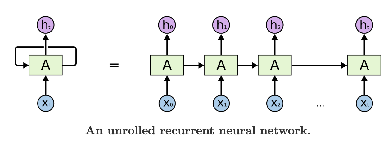
RNNs are usually used for data that are in sequence and lists. For example, speech recognition, translation, image captioning, etc.
A more detailed look at the recurrent layer and an unfolded RNN with 3 time stamps:
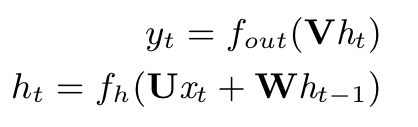
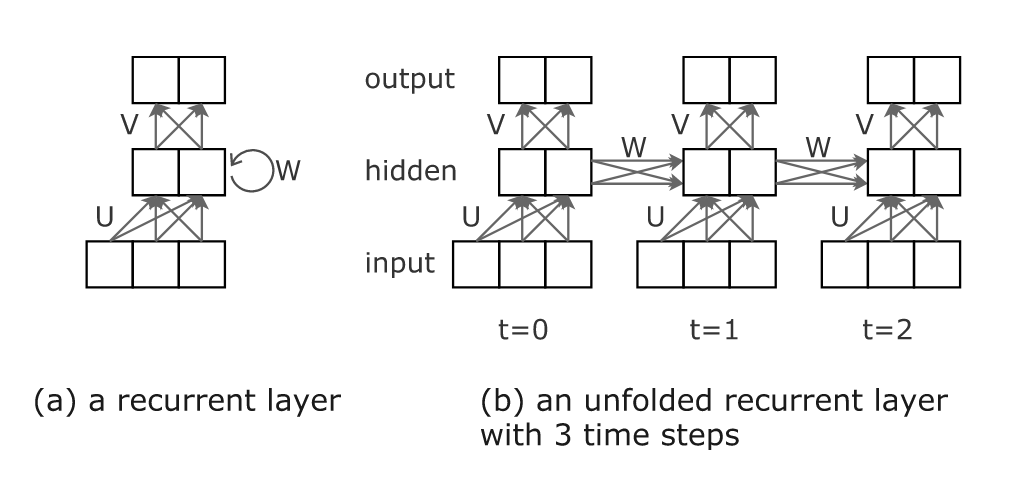 Choi et al., 2018, p. 8
-
fout is usually soft-max/sigmoid, etc.
-
fh is usually tanh or ReLU
-
ht is hidden vector of the network that stores info at time t
-
U, V, W are matrices with trainable weights of the recurrent layer
Sequence-to-Sequence Encoder-Decoder RNNs
Here let’s use the example of machine translation.
- We first use a tokenizer to break the sentences into tokens
- Tokens are turned into word embeddings.
- We could either train our own word embeddings or use a pre-trained embedding
- We could either train our own word embeddings or use a pre-trained embedding
- Pass the word embeddings into the encoder RNN, one word at a time. For the next word, we pass in the hidden state of the last word and the next word embedding.
- Pass the last hidden state into the decoder RNN. The last hidden state is called context.
- The decoder also has a hidden state that is not shown in the visualization below.
- The context is what made RNN bad at dealing with long sequences, because it only contains the last hidden state
Video below shows an unrolled RNN neural translator.
Use ATTENTION to enhance sequence-to-sequence encoder-decoder RNNs
Instead of looking at only the last hidden state, we look at all encoder hidden states. At each time stamp, we incorporate an attention step before output. Attention tells the model a specific component to pay attention to.
Attention
- Look at all encoder hidden states (usually an encoder hidden state is most associated with a certain word)
- Give all hidden states a score (not explained)
- Transform the scores with softmax
- Multiply the original hidden states with the softmaxed score
- Sum up the weighted hidden states to obtain context vector for the current decoder
Incorporating Attention in the Encoder-Decoder Model
Steps only applicable to the first decoder cycle
- The attention decoder takes in the embedding of the
token and initial decoder hidden state - Produces a new decoder hidden state at the current timestamp (in the illustration below it is timestamp 4) and discards its output.
Below steps can be repeated at each timestamp
- The RNN processes the inputs (previous decoder hidden state + ouput from previous step) to get the current decoder hidden state
- Attention step from above: uses all encoder hidden states and the current decoder hidden state (h4) to calculate a context vector (C4)
- Concatenate context vector (C4) with the current hidden state (h4) into one vector
- Feed this one vector into a feedforward neural network (it is trained jointly with the model)
- Output of the feedforward neural network indicaates the output word of this time step.
- Repeat for the next time steps
LSTM (Long Short Term Memory)
LSTM is a special kind of RNN. The additive connections between time-steps help gradient flow, remedying the vanishing gradient problem (see below for where the additive connections come from in LSTM)
Standard RNNs handle short term dependencies pretty well, but not long term dependencies. LSTM handles this long term dependency.
-
Short Term Dependency Example: clouds in the [] <- it’s easy for RNN to predict sky
-
Long Term Dependency Example: I grew up in France.(…) I speak [] <- hard for RNN to predict French
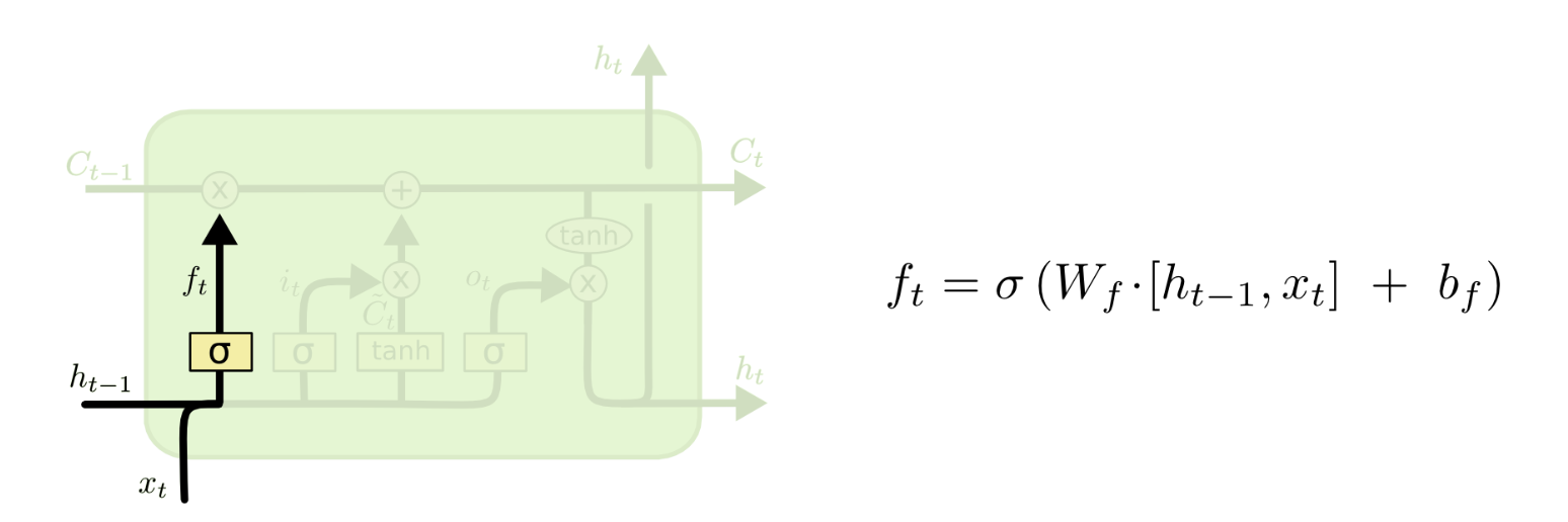
Inside the LSTM unit (a “cell”), there are gates (forget gate, input gate, and output gate). There are also states: hidden state and cell state. We’ll look at the LSTM unit step by step.
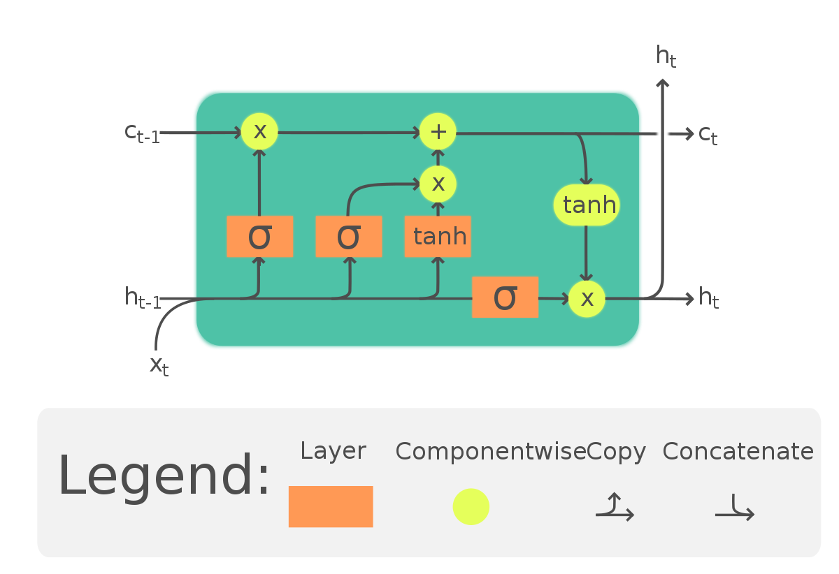
Terminology Alert!**
Hidden state: (in both standard RNN and LSTM)
- Working memory capability that carries information from immediately previous events and overwrites at every step uncontrollably
Cell state: (only in LSTM)
-
Long term memory capability that stores and loads information of not necessarily immediately previous events
-
Can be considered at a conveyor belt that carries the memory of previous events
Gates:
“A gate is a vector-multiplication node where the input is multiplied by a same-sized vector to attenuate the amount of input.”
The three gates mentioned above usually contains a sigmoid layer coupled with tanh layer. The sigmoid layer returns a value between (0,1) that determines what part of data needs to be forgotten, updated, and outputted. Remember they have different weights (see formula below.)
Step 1: Forget Gate Layer - Determine what information to forget
It is worth noting that we are not actually doing the forgetting here. We are only running the previous hidden state and the current input date through a sigmoid layer and decide what information to forget.
Example: The store owner saw the little girl. We might want to forget the gender pronoun of the store owner here to update it with the little girl’s. Step 1 is to decide we are forgetting store owner’s gender.
Step 2: Input Gate Layer - Determine what information to update and store in our cell state
The sigmoid layer determines which values we update. Tanh layer transforms the input layer into the range between (-1,1). We still have not combined these two layers to create an update to the cell state yet.
Example: The store owner (he) saw the little girl. She was looking at candy bars. We need to determine that we need to add in the gender pronoun of the little girl. 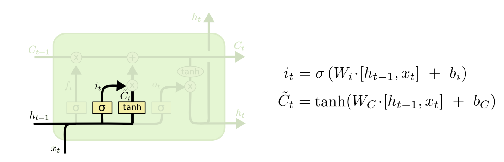
Step 3: Cell State Update - element-wise operation to make updates
Now we take the information that we’ve determined to forget during the forget gate layer and apply it to the cell state. Then we multiply the input gate sigmoid layer with the newly transformed values from tanh layer and add it to our cell state. 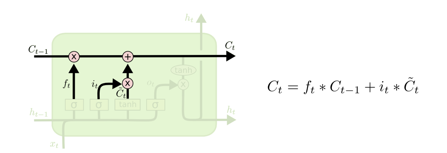
Step 4: Output Gate Layer - Determine what we are outputting
Similar to the structure of the input gate layer, the output gate layer also consists of two parts: sigmoid layer to determine what information to output, and tanh layer to transform the cell state data to have a range of (-1,1). Then we multiply them and output the transformed value of the data that we want the model to output. 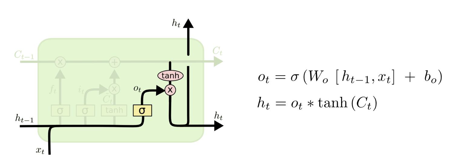
Recurrent Layers and Music
Shift invariance cannot be incorporated in the computation inside recurrent layers, so recurrent layers may be suitable for the sequence of features.
The number of hidden nodes in a layer is one of the hyperparametes and can be chosen through trial and error.
Length of the recurrent layer can be controlled to optimize the computational cost. Onset detection can use a short time frame, whereas chord recognition may benefit from longer inputs.
For many MIR problems, inputs from the future can help the prediction, so bi-directional RNN can be worth trying. We can think of it as having another recurrent layer in parallel that works in the reversed time order.
Solving MIR Problems: Practical Advice
Data Preprocessing
-
It’s crucial to preprocess the data because it affects the training speed.
-
Usually logarithmic mapping of magnitudes is used to condition the data distributions and result in better performance
-
Some preprocessing methods did not improve model performance:
-
spectral whitening
-
normalize local contrasts (did not work well in CV)
-
-
Optimize the signal processing parameters such as the number of FFTs, mel bins, window and hop sizes, and the sampling rate.
- Audio signals are often downmixed and downsampled to 8-16Hz
Aggregating information
-
Time varying problems, which are problems with a short decision time scale (chord recognition, onset detection) require a prediction per unit time
-
Time invariant problems, which are problems with a long decision time scale (key detection, music tagging), require a method to aggregate features over time. Methods are listed as below:
-
Pooling: common example would be using max pooling layers over time or frequency axis
-
Strided convolutions: convolutional layers that have strides bigger than 1. The effects are similar to max pooling, but we should not set strides to be smaller than kernel size. Otherwise not all of the input will be convolved.
-
Recurrent layers: can learn to summarize features in any axis, but it takes more computation and data than the previous two methods. So it is usually used in the last layer.
-
Depth of networks
-
Bottom line is that the neural network should be deep enough to approximate the relationship between the input and the output
-
CNNs have been increasing in both MIR and other domains, which is also allowed by recent advancement in computational savings.
-
RNNs have increased slowly because 1) stacking recurrent layers does not incorporate feature hiearchy and 2) recurrent layers are already deep along the time axis, so depth matters less