Deep Learning for Music Information Retrieval – Pt. 2
This series is inspired by my recent efforts to learn about applying deep learning in the music information retrieval field. I attended a two-week workshop on the same topic at Stanford’s Center for Computer Research in Music and Acoustics, which I highly recommend to anyone who is interested in AI + Music. This series is guided by Choi et al.’s 2018 paper, A Tutorial on Deep Learning for Music Information Retrieval.
It will consist of four parts: Background of Deep Learning, Audio Representations, Convolutional Neural Network, Recurrent Neural Network. This series is only a beginner’s guide.
My intent of creating this series is to break down this topic in a bullet point format for easy motivation and consumption.
Music Information Retrieval
Background of MIR
-
Usually means audio content, but also extends to lyrics, music metadata, or user listening history
-
Audio can be complemented with cultural and social background like genre or era to solve MIR topics
-
Lyric analysis is also MIR, but might not have much to do with audio content
Problems in MIR
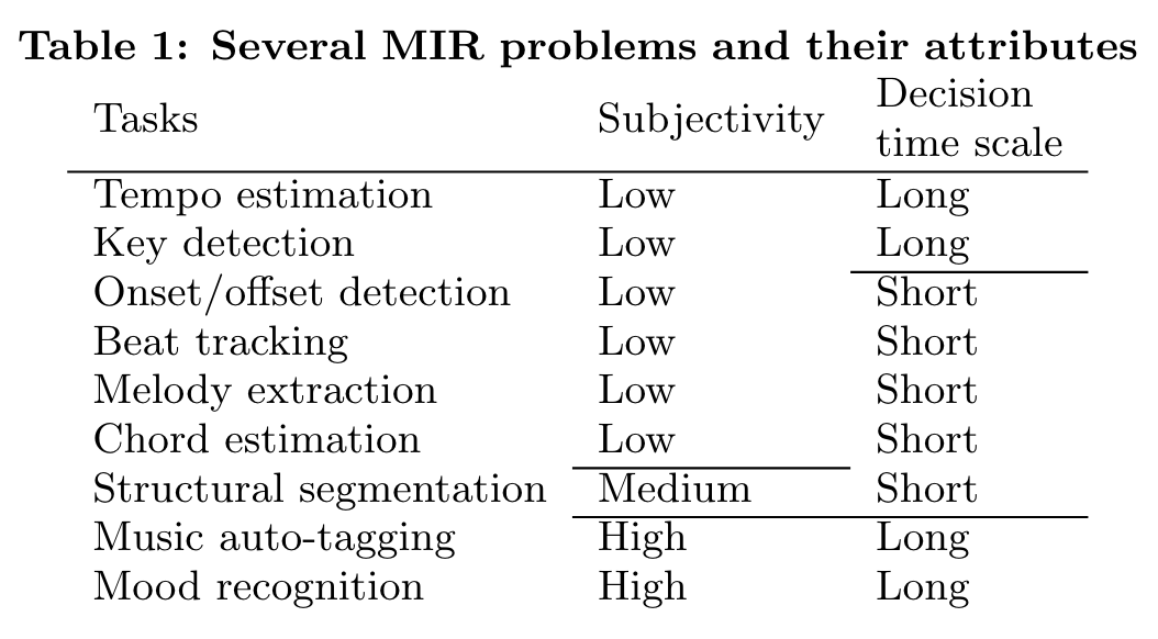 Choi et al., 2018, p.6
Subjectivity
-
Definition: Absolute ground truth does not exist
-
Example: music genres, the mood for a song, listening context, music tags
-
Counter example: pitch, tempo are more defined, but sometimes also ambiguous
-
Why deep learning has achieved good results: it is difficult to manually design useful features when we cannot exactly analyze the logic behind subjectivity
Decision Time Scale
-
Definition: unit time length the prediction is made on
-
Example:
-
Long decision time scale (time invariant problems): tempo and key usually do not change in an excerpt
-
Short decision time scale (time-varying problems): melody extraction usually uses time frames that are really short
-
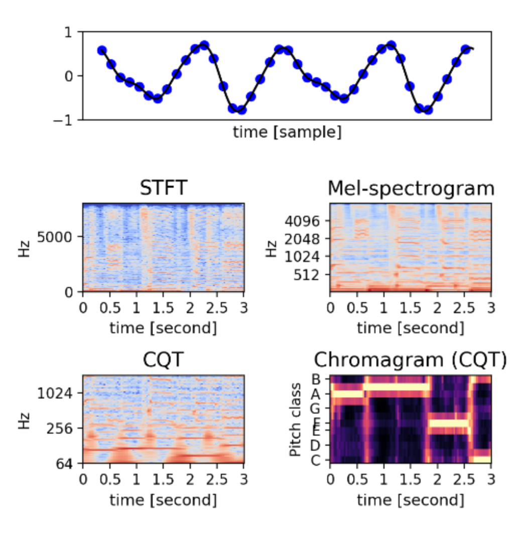
Audio Data Representations
-
General background: audio signals are 1D, time-frequency representations are 2D and have a couple of options (listed below)
-
Important to pre-process the data and optimize the effective representation of audio data to save computational costs
-
2D representations can be considered as images but there are differences between images and time-frequency representations
-
Images are usually locally correlated (meaning nearby pixels will have similar intensities and colors)
-
But spectrograms are often harmonic correlations. Their correlations might be far down the frequency axis and the local correlations are weaker
-
Scale invariance is expected for visual object recognition but probably not for audio-related tasks.
- Here scale invariance means if you enlarge a picture of a cat, the model will still be able to recognize that it’s a cat.
-
 Choi et al., 2018, p.6
Audio Signals
-
Samples of the digital audio signals
-
Usually not the most popular choice, considering the sheer amount of data and the expensive cost of computation
- Sampling rate is usually 44100 Hz, which means one second of audio will have 44100 samples
-
But recently one-dimensional convolutions can be used to learn an alternative of existing time-frequency conversions
Short Time Fourier Transform
-
Definition: The procedure for computing STFTs is to divide a longer time signal into shorter segments of equal length and then compute the Fourier transform separately on each shorter segment.
-
(+) Computes faster than other time-frequency representations thanks to FFTs
-
(+) invertible to the audio signal, thus can be used in sonification of learned features and source separation
-
(-) its frequencies are linearly centered and do not match the frequency resolution of human auditory system -> mel spectrogram is
-
(-) not as efficient in size as mel sepctrogram (log scale), but also not as raw as audio signals
-
(-) it is not musically motivated like CQT
Mel Spectrogram
-
2D representation that is optimized for human auditory perception.
-
(+) It compresses the STFT in frequency axis to match the logarithmic frequency scale of human hearing - hence efficient in size but preserves the most perceptually important information
-
(-) not invertible to audio signals
-
Popular for tagging, boundary detection, onset detection, and learning latent features of music recommendation due to its close proximity to human auditory perception.
Constant-Q Transform (CQT)
-
Definition: It is also a 2D time-frequency representation that provide log-scale centered frequencies. It perfectly matches the frequency distribution of pitches
-
(+) Perfectly matches the pitch frequency distribution so it should be used where fundamental frequencies of notes should be identified
- Example: Chord recognition and transcription
-
(-) Computation is heavier than the other two
Chromagram
-
Definition: Pitch class profile, provides the energy distribution on a set of pitch class (from C to B)
-
It is more processed than other representations and can be used as a feature by itself, just like MFCC