Deep Learning for Music Information Retrieval – Pt. 1
This series is inspired by my recent efforts to learn about applying deep learning in the music information retrieval field. I attended a two-week workshop on the same topic at Stanford’s Center for Computer Research in Music and Acoustics, which I highly recommend to anyone who is interested in AI + Music. This series is guided by Choi et al.’s 2018 paper, A Tutorial on Deep Learning for Music Information Retrieval.
It will consist of four parts: Background of Deep Learning, Audio Representations, Convolutional Neural Network, Recurrent Neural Network. This series is only a beginner’s guide.
My intent of creating this series is to break down this topic in a bullet point format for easy motivation and consumption.
Brief Context on Deep Learning
Development history of Neural Networks
-
Error backpropagation: way to apply the gradient descent algorithm for deep neural networks
-
Convolutional neural network was introduced to recognize handwritten digits.
-
Long short-term memory recurrent unit was introduced for sequence modelling.
- Sequence models input and output streams of data. For example, text streams and audio clips. Applications include speech recognition, sentiment classification, and video activity recognition
Recent Advancements that Contributed to Modern Deep Learning
-
Optimization technique: Training speed has improved by using rectified linear units (ReLUs) instead of sigmoid functions
-
Parallel computing on graphical computing units (GPUs) also encourages large-scale training
Deep Learning vs Conventional Machine Learning
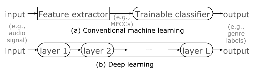 Diagram for Conventional Machine Learning vs Deep Learning
 Conventional machine learning
-
Hand designing the features & the machine learning a classifier
-
Using MFCCs as inputs to train a classifier because we already know that MFCC can provide relevant information for the task
-
Only part of the model learns from the data (classifier part), the MFCCs are calculated by us and not learned by the model from the data
-
Deep Learning
-
Both the feature extraction and the classifier part comes from the model.
-
Having multiple layers coupled with the nonlinear activation functions allows the model to learn complicated relationships between inputs and outputs
-
Input and output might not be directly correlated. For example, input can be audio signals but output can be genres.
-
When to use Deep Networks?
-
When there are at least 1000 samples. Samples here do not necessarily mean number of tracks, it should be specific to the task that you are performing.
- For example, you don’t need a lot of tracks to train a model on chord recognition - as long as you have enough chords in those tracks
What to do if there’s not enough data?
-
Data augmentation: adding some sort of distortion while preserving the core properties. This step is also highly dependent on task.
-
Example: time stretching and pitch scaling for genre classification
-
Note that this will not work for key or tempo detection
-
-
Transfer learning: reusing a network that is previously trained on another task(source task) for current task (target tasks)
-
Assuming that there are similarities in the source task and target tasks, so that the pre-trained networks can actually provide relevant representations
-
The pre-trained network serves as a feature extractor and learns a shallow classifier
-
-
Random Weights Network: also known as networks without training.
-
Network structure is built based on a strong assumption of the feature hierarchy, so the procedure is not completely random
-
Similar to transfer learning, random weights network also can serve as a feature extractor
-
Designing & Training a Deep Neural Network
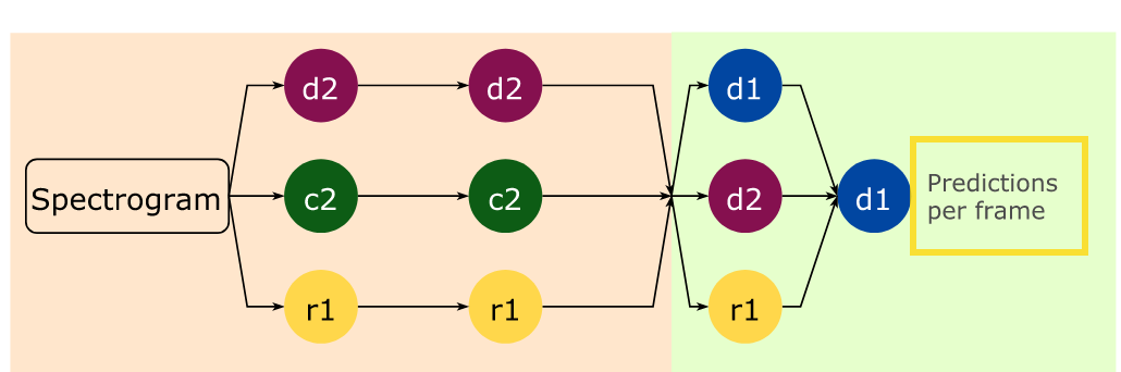 Sneak peek of the overall structure of a deep neural network with 3 hidden layers.
 Here we assume you have a basic understanding of what a standard neural network looks like and how forward propagation and back propagation works. If not, I recommend this 12-min long video by Andrew Ng.
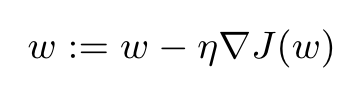
Gradient Descent
-
Training speed affects the overall performance because a significant difference on the training speed may result in different convergences of the training. We need to control the learning rate and the gradient smartly to optimize the training speed.
-
Learning rate η: can be adaptively controlled. When it is far away from local minima, our gradient should take big steps, but when it gets closer, it should take smaller steps.
- ADAM is an optimizer that uses learning rate. It is an extension to the stochastic gradient descent
-
Gradient ∇J(w): due to backpropagation, gradient at l-th layer is affected by the gradient at l +1th layer.
-
Reminder on different types of gradient descent algorithms: batch Gradient Descent, Mini-batch Gradient Descent, Stochastic Gradient Descent
Activation functions
Why do we need activation functions?
Activation functions determines whether or not a node is considered to be activated or deactivated.
We also use it to add nonlinearity into our model. We need nonlinearity because real world data is complex and cannot be captured only through a linear model. It is also worth noting that without a non-linear activation function in the network, a NN, no matter how many layers it had, would behave just like a single-layer perceptron, because summing these layers would give you just another linear function.
sigmoid vs tanh vs ReLU vs leaky ReLU and softmax
Sigmoid: output range (0,1) 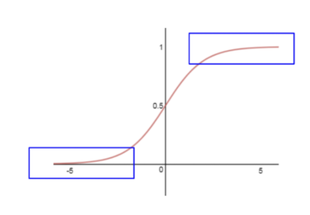
-
Not centered around zero, all its output are positive.
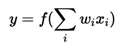 f here is the sigmoid activation function.
We have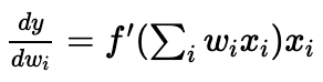 as the gradient. Because xi (output from sigmoid layer) is always positive, the gradient is also always either positive or negative. But to get the optimum value, weights sometimes take on opposite signs. This will cause zig zag behavior.
 -
In the blue box, the gradient vanishes when the input values are too big or too small (vanishing gradient problem)
Tanh: output range (-1,1)
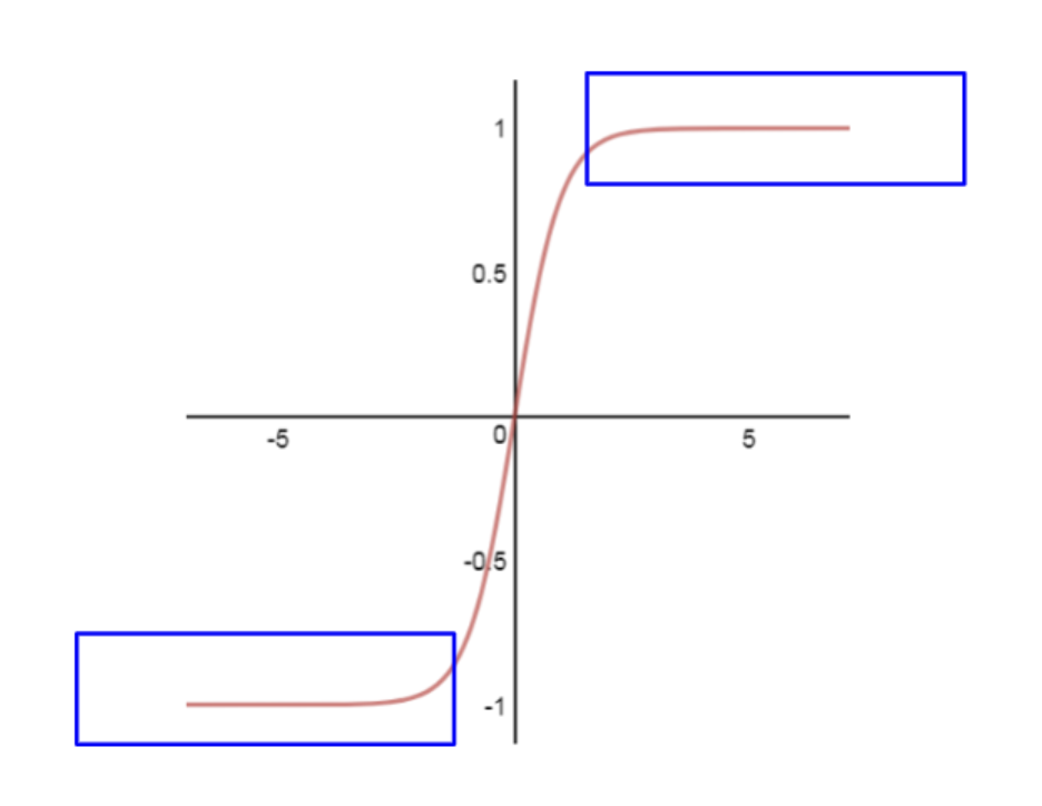
Similar to sigmoid, it also has the vanishing gradient problem. But it is zero centered.
ReLU - output range: [0, infinity)
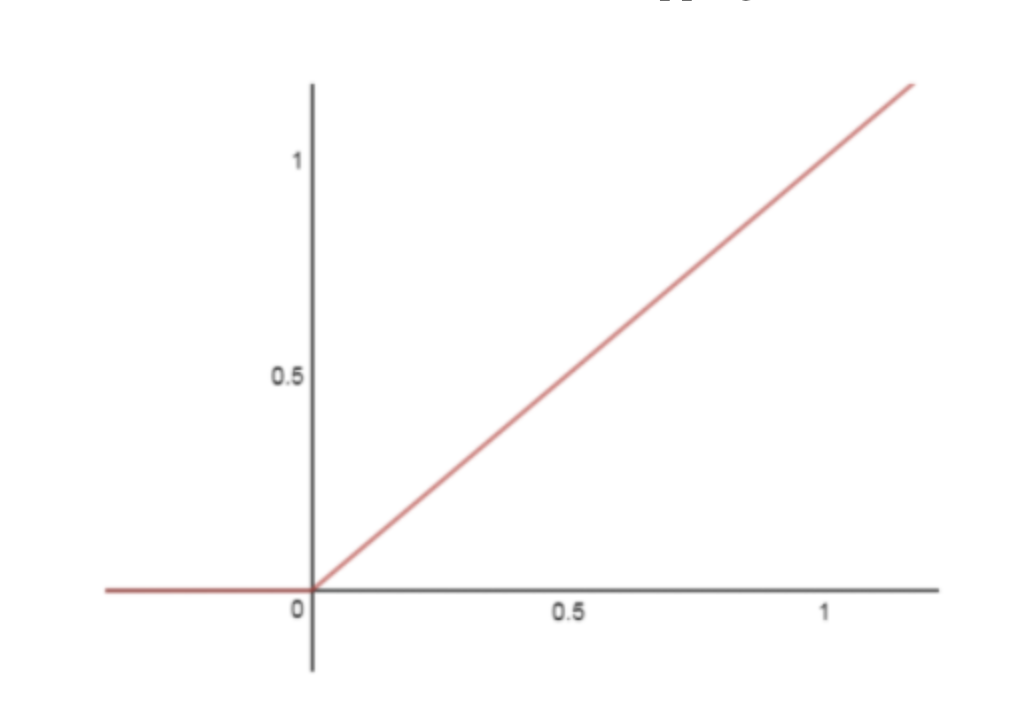
R(x) = max(0, x)
(+) Faster to converge compared with other activation function. Computationally inexpensive.
(-) It’s likely when we are updating the weights, the output of a neuron is always x<0. Hence, ReLU always sets it to 0. If this happens, the neuron just never gets activated and does not make contributions.
Leaky ReLU
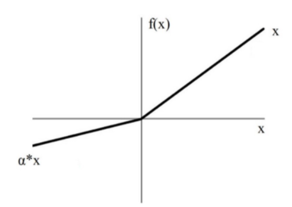
Instead of the standard ReLU, it adds a parameter alpha that avoids having a “dead” neuron.
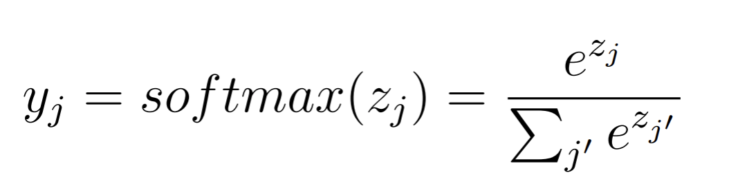
Softmax
Softmax is only applied in the last layer to predict probability values in classification tasks.
The input vectors need to be mutually exclusive, and the probability output needs to sum up to 1.
Deep Neural Networks for MIR
This series will also cover convolutional neural network (part 3) and recurrent neural network (part 4) in details. Here we briefly discuss dense layers.
Dense Layers in Music
Choi et al., 2018, p. 6 There could be dense layer that only looks at the current frame like d1, but there could also be dense layers with contexts that look at multiple frames like d2.
-
Note: A dense layer does not facilitate a shift or scale invariance.
-
Example: A STFT with frame length of 257 will be mapped from 257 dimensional space to a V-dimensional space (where V is the number of nodes in a hidden layer)
-
Even a tiny shift in frequency will be a different representation in
-
-
We usually combine dense layers with CNNs or RNNs for various MIR tasks.
Resources:
Stackoverflow answer about why we need nonlinearity in Neural Network here